Free Cooling Chiller Payback: Annual Operating Cost Guide
Technical guide · September 30, 2026
A free cooling chiller (also called a natural cooling chiller) is worth evaluating when your facility needs cooling during hours when outdoor air, through a dry cooler or integrated free cooling coil, can carry some or all of that load. The purchasing decision then comes down to a second question: does the reduction in compressor electricity exceed the additional fan, pump, maintenance and installation costs over the owner’s evaluation period?
Answering that question requires a weather-and-load comparison. A count of cold days, a peak efficiency rating or a supplier’s annual savings percentage cannot establish the result for your facility.
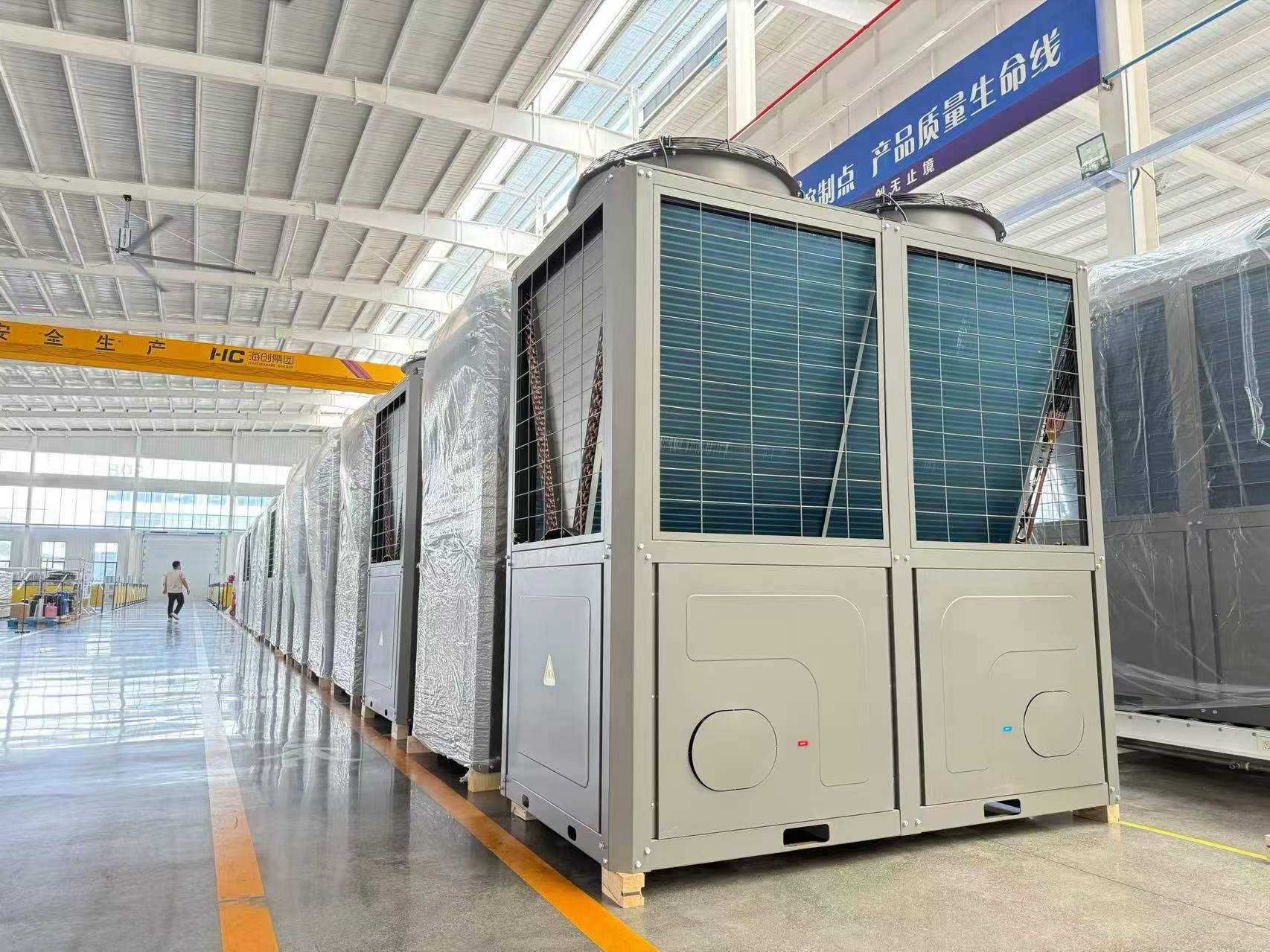
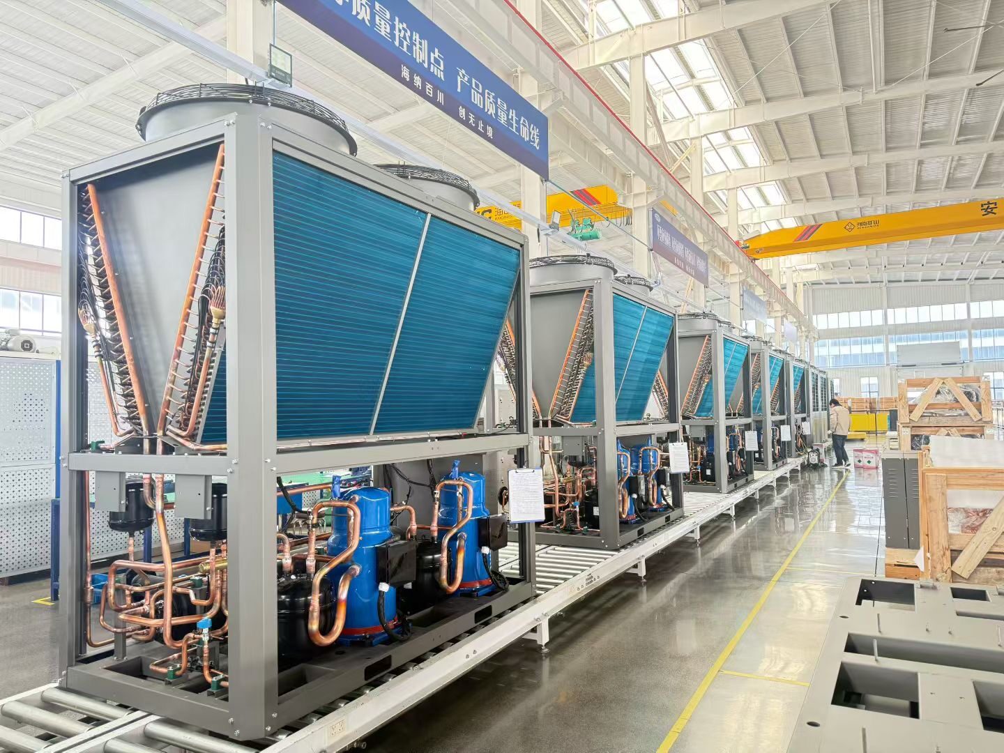
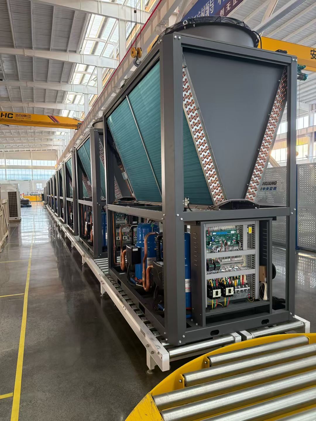
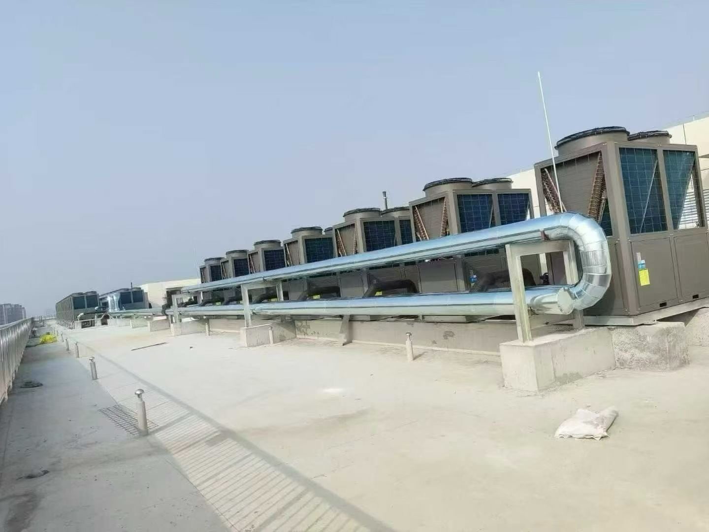
This guide focuses on chillers with an ambient-air free cooling circuit, commonly serving process facilities and technical cooling applications. SongXin’s natural cooling chiller range describes mechanical, hybrid and natural cooling operation. The method below helps turn those operating modes into a comparable enquiry and a transparent cost estimate.
Key takeaways
- Outdoor air colder than the return fluid creates an opportunity for partial free cooling. Full free cooling also needs enough heat-exchanger capacity to reach the supply setpoint at the required load.
- Each additional 1 K of heat-exchanger approach, including an intermediate plate heat exchanger, lowers the outdoor-temperature ceiling for full free cooling by about 1 K at the selected duty. The effect on annual hours depends on local weather and load.
- Compare total electrical input, including extra pump and fan power, against a conventional chiller that also unloads in mild weather.
- In the worked example, a US$85,000 premium pays back in 5.0 years, but 12.4 years if half the mild and cold operating hours disappear.
About the examples in this guide: All numbers in the worked examples are fictional assumptions chosen to demonstrate the method. They are not typical values, design allowances, or measured SongXin performance. Use the selected equipment’s data and your project conditions for any real decision. In formulas, x means multiplication and ~= means approximately equal.
When Does a Free Cooling Chiller Actually Save Energy?
A free cooling chiller saves electricity when the reduction in compressor input exceeds the added fan and pump input while meeting the same cooling duty. An integrated unit can use outdoor air to precool the returning fluid while refrigeration supplies the remaining duty. As outdoor temperature falls, it can progress from mechanical, through partial, to full free cooling.
The distinction matters because starting free cooling and meeting the complete load without compressors are different operating points. Outdoor air colder than the return fluid creates a useful temperature difference; it does not, by itself, prove that the heat exchanger can deliver the specified supply temperature at the required load.
Ask the supplier to identify three results at each relevant operating point:
- Available free cooling capacity at the stated ambient temperature, fluid temperatures, flow and fluid composition.
- The remaining duty assigned to the refrigeration circuit.
- Total electrical input with the proposed fan, pump and compressor control sequence.
Use the actual circuit diagram. A dry air-to-fluid heat exchanger is evaluated against outdoor dry-bulb conditions, while an evaporative cooling-tower economizer uses a different temperature basis. A tower-based example is useful for understanding load coincidence and system power, but its wet-bulb thresholds should not be copied into a dry-cooler selection.
How Chilled Water Temperature Sets Your Free Cooling Hours
Before counting eligible hours, calculate the temperature difference the proposed heat exchangers actually need. This is often the assumption that changes the investment decision most.
When Does Partial Cooling Become Full Free Cooling?
For a dry air-to-fluid exchanger, define the leaving-fluid approach as:
Approach = fluid temperature leaving the free cooling coil - entering outdoor-air temperatureThis approach is a result at a particular flow, load, fluid mixture and fan setting. It is not a permanent property that stays unchanged across the year. A colder outdoor temperature increases the available temperature difference, but the exchanger still has finite capacity.
In this fictional thermal example, use water at 12 kg/s, a specific heat of 4.18 kJ/(kg·K), and a required 23°C return / 18°C supply schedule:
Delivered cooling duty = mass flow x specific heat x temperature difference
                       = 12 x 4.18 x (23 - 18)
                       = 250.8 kW
The selection has these operating points:
REFERENCE TABLE · Scroll horizontally on smaller screens to read all columns.
| Outdoor air | Fluid leaving the free cooling stage | Free cooling contribution | Remaining refrigeration duty | Meaning |
|---|---|---|---|---|
| 22°C | Stage bypassed; 23°C | 0 kW | 250.8 kW | No useful operation is assumed for this selected point |
| 17°C | 20°C | 12 × 4.18 × 3 = 150.5 kW | 100.3 kW | Useful partial cooling, but the fluid still needs cooling to 18°C |
| 12°C | Controlled to 18°C | 250.8 kW | 0 kW | The selected free cooling stage meets the complete duty |
The results distinguish heat removed from the return stream from meeting the specified supply condition. At 17°C outdoors, the partial contribution is about 60% of the load even though compressors remain necessary.
If the selected dry coil needs a 3 K approach at the full-duty point, 18°C supply would require outdoor air no warmer than approximately 15°C. That temperature is a screening boundary; the capacity and fan selection must still support it. If an intermediate plate heat exchanger adds an assumed 2 K terminal approach, the corresponding screen moves to approximately 13°C. Both approach assumptions need confirmation at the actual duty.
This is why a glycol-isolated arrangement can have fewer full free cooling hours than a direct circuit with otherwise similar components. Isolation may be valuable for the building loop, but it introduces another temperature difference, hydraulic circuit and potentially another pump. Compare the complete arrangements.
Can the Process Accept a Higher Chilled Water Temperature?
A process that accepts 18°C fluid offers a different free cooling opportunity from equipment that requires 7°C. However, raising the supply setpoint is a system decision. Check the process heat exchanger’s required approach, maximum equipment inlet temperature, terminal cooling capacity and any humidity duty. A chilled-water reset that helps the chiller can reduce dehumidification at a cooling coil.
Also examine the return temperature at the real flow. Excess flow can reduce the water temperature rise for a given load, weakening the return-to-ambient temperature difference. It is therefore possible for a poorly balanced system to have attractive weather data but less usable partial cooling than the proposal assumes. Use measured return temperatures where available, and distinguish them from the design temperature printed on the original schedule.
How to Count Useful Free Cooling Hours
A facility that stops production on winter nights cannot count those hours as useful free cooling hours. Conversely, a technical cooling load that continues overnight may coincide with favorable outdoor conditions even when daytime temperatures are high.
Build an hourly schedule where possible. For an initial assessment, group hours into sufficiently narrow temperature and load bands, then request performance at representative points within each band. The waterside economizer application guidance uses coincident weather and load data to assess operating opportunities. The useful principle is to pair the conditions; the equipment configuration still determines the applicable temperature and performance model.
For every hour or band, record:
REFERENCE TABLE · Scroll horizontally on smaller screens to read all columns.
| Input | What the project team should provide | Why it changes the comparison |
|---|---|---|
| Cooling demand | Required delivered cooling in kW, including shutdown periods | Cold weather has no cooling value when there is no demand |
| Fluid temperatures | Required supply temperature and expected return temperature | These determine the thermal duty available to the free cooling circuit |
| Outdoor conditions | Relevant weather data and equipment inlet-air conditions | The heat exchanger must operate at the actual heat-rejection condition |
| Fluid and flow | Water or named glycol mixture, concentration and flow | Both equipment capacity and hydraulic losses must match the selected fluid |
| Operating schedule | Production, occupancy, night operation and seasonal shutdowns | This establishes the hours to which each power input applies |
| Plant availability | Equipment staging, standby requirements and maintenance periods | An unavailable circuit cannot contribute modeled savings |
Keep the same delivered cooling requirement for both proposals. Raising the chilled-water temperature in only the free cooling option creates a different comparison. If the process or terminal equipment can accept a warmer schedule, evaluate that schedule in both options and verify that the end-use requirement is still met.
For projects where the cooling duty or fluid conditions are not yet established, complete the industrial process chiller selection brief first. The annual cost model needs that design basis. If the heat-rejection arrangement is still open, use the air-cooled vs water-cooled chiller selection guide to establish the plant boundary before comparing hourly input.
Include Pump and Fan Power in the Comparison
Write the comparison boundary at the top of the cost sheet. For example:
Chiller package, including its fans and compressors, plus all pumping required to deliver cooling at the agreed system connection.
Then list any equipment outside that boundary separately. If package input already includes the free cooling fans, do not add them again. If it excludes an external pump, include that pump explicitly.
Request separate pressure losses with free cooling active and inactive, together with mode-specific pump duty. The additional hydraulic path can change pumping input even when the delivered cooling requirement is unchanged.
A proposal described as “glycol free” also needs a circuit drawing. Establish which loop contains which fluid, whether an intermediate heat exchanger is present, and how each exposed circuit is protected during operation and shutdown. Use the offered equipment’s fluid limits and protection requirements for each circuit.
How Much Pump Power Does Free Cooling Add?
For a first estimate at a known operating point:
Pump electrical input, kW
= volumetric flow, m^3/s x pressure rise, Pa / (1,000 x overall efficiency)
Overall efficiency here includes the pump, motor and any drive losses. This fluid-power accounting is consistent with the system approach in the US Department of Energy pumping sourcebook. Use the selected pump’s performance at each operating point for the final assessment.
In this fictional pump example, assume 0.012 m³/s, an additional 60,000 Pa of resistance when the free cooling path is active, and unchanged overall efficiency of 0.60:
Additional input ~= 0.012 x 60,000 / (1,000 x 0.60) = 1.2 kW
At 5,500 active hours: 1.2 x 5,500 = 6,600 kWh/year
The estimate holds flow and efficiency constant. A fixed-speed pump may instead move to a different flow. A controlled pump may raise speed, and its efficiency can change. The final comparison needs the resulting flow, pressure and electrical input together. Do not add this estimate again where the annual model already includes the corresponding pump input.
Fluid composition also belongs in the thermal selection. The relationship Q = mass flow × specific heat × temperature difference means that a change in specific heat changes the required mass flow for the same duty. Density converts that mass flow to volume flow; viscosity affects pressure loss and exchanger performance. Request properties for the named mixture at the relevant temperature, rather than using the water calculation above for a glycol circuit.
Hybrid Mode at Low Load: Compressor Minimum Capacity
A thermally useful free cooling stage does not guarantee that the combined package has a stable or economical operating point. The refrigeration circuit also has minimum capacity, flow and run-time constraints.
In this fictional low-load example, assume an 80 kW building load, 65 kW available free cooling and a refrigeration circuit with a minimum stable output of 35 kW. Subtracting the free contribution leaves only 15 kW for refrigeration. Simply running both stages at those stated capacities would not balance the load. One possible strategy is to limit free cooling to 45 kW while refrigeration supplies 35 kW; other equipment may use different staging, cycling or storage arrangements.
The supplier must demonstrate the sequence appropriate to its package. Compare total input at the resulting stable point with mechanical-only operation. Do not automatically choose the mode that removes the most heat through the free cooling coil if its additional fan and pump input outweighs the compressor reduction.
Request a mode table that covers the following transitions:
REFERENCE TABLE · Scroll horizontally on smaller screens to read all columns.
| Operating event | What the sequence must establish |
|---|---|
| Free cooling becomes available | Valid sensor readings, proven circulation, valve positions and a useful capacity or power advantage |
| Partial cooling increases | Refrigeration unloading remains inside its allowed operating range while supply temperature stays within the process limit |
| Compressors stop | Free cooling can sustain the load and supply setpoint; a momentary favorable sensor value is insufficient |
| Load rises or ambient temperature increases | Refrigeration returns before the process temperature limit is exceeded |
| Conditions hover near a threshold | Separate enable/disable conditions or another documented anti-cycling strategy prevent repeated mode changes |
| A pump, sensor or free cooling circuit becomes unavailable | The fallback sequence has a defined available capacity and an alarm the operator can act on |
Include freeze protection during shutdown and loss of power in the design discussion. Circulation or electric heating that depends on an energized supply cannot be treated as passive protection during an outage. The selected fluid, exposed components and approved protection sequence must be considered together.
Worked Example: Annual Savings and Payback
In this fictional annual example, a facility operates for 8,000 cooling hours per year. It has 760 other hours with no cooling requirement; standby electricity is assumed equal between options and is excluded. Within each operating band, the listed load and power are treated as constant. A real assessment should use finer bands or hourly calculations where variation is material.
Both options meet the same fluid-temperature schedule and the same load in each row. “Package input” includes all fans and compressors inside the selected package. Pumping is additional.
REFERENCE TABLE · Scroll horizontally on smaller screens to read all columns.
| Assumed operating band | Cooling duty | Annual hours | Conventional package + pumps | Free cooling proposal: package + pumps | Total input difference |
|---|---|---|---|---|---|
| Warm; mechanical operation | 350 kW | 2,500 h | 105 + 10 = 115 kW | 106 + 12 = 118 kW | 3 kW more |
| Mild; hybrid operation | 280 kW | 3,500 h | 75 + 8 = 83 kW | 44 + 10 = 54 kW | 29 kW less |
| Cold; full free cooling | 220 kW | 2,000 h | 50 + 6 = 56 kW | 12 + 10 = 22 kW | 34 kW less |
The conventional chiller is assumed to use less power in colder, lower-load conditions too. Comparing free cooling against a baseline that remains at summer peak power all year would overstate the benefit.
Calculate annual electricity as the sum of total input in kW × operating hours:
Conventional system:
(115 x 2,500) + (83 x 3,500) + (56 x 2,000)
= 690,000 kWh/year

Free cooling proposal:
(118 x 2,500) + (54 x 3,500) + (22 x 2,000)
= 528,000 kWh/year

Difference:
690,000 - 528,000 = 162,000 kWh/year
The assumed warm-weather penalty is 7,500 kWh. Savings in the mild and cold bands are 101,500 and 68,000 kWh respectively. Keeping all three contributions visible prevents the attractive cold-weather result from hiding a penalty elsewhere.
Assume an electricity price of US$0.12/kWh, additional maintenance of US$2,440/year, and an additional installed cost of US$85,000:
Electricity-cost saving = 162,000 x 0.12 = US$19,440/year
Net annual saving = 19,440 - 2,440 = US$17,000/year
Simple payback = 85,000 / 17,000 = 5.0 years
This is a screening calculation. It excludes demand charges, financing, discounting, tariff escalation, tax effects and future component replacement. Add those items when they influence the owner’s decision. In particular, winter electricity savings do not automatically reduce a demand charge set by a summer peak.
Sensitivity Check: What If Operating Hours Are Lower?
An attractive result is useful only if its decisive inputs are credible. Start with the operating schedule.
Suppose the same facility operates for only half the mild and cold hours, while retaining all 2,500 warm hours. Keep the assumed power differences unchanged during the remaining hours:
Revised electricity saving:
-(3 x 2,500) + (29 x 1,750) + (34 x 1,000)
= 77,250 kWh/year

Revised net annual saving:
(77,250 x 0.12) - 2,440 = US$6,830/year

Revised simple payback:
85,000 / 6,830 ~= 12.4 years
The investment case changes because fewer operating hours coincide with useful free cooling conditions.
Other useful sensitivities include a different electricity tariff, a lower permitted fluid temperature, a change in production load and higher pumping power. Change each assumption in the model rather than applying an unexplained percentage reduction to the predicted saving.
How Many Operating Hours Meet an Eight-Year Payback Target?
The same annual example can be used backwards. Suppose the owner sets an assumed maximum simple payback of eight years, retaining the US$85,000 premium, US$2,440 additional maintenance and US$0.12/kWh tariff:
Required net annual saving = 85,000 / 8 = US$10,625
Required electricity saving = (10,625 + 2,440) / 0.12
                             = 108,875 kWh/year
If the 2,000 cold hours and 2,500 warm hours remain credible, let H be the required mild-band hours:
29 x H + (34 x 2,000) - (3 x 2,500) >= 108,875
H >= (108,875 - 68,000 + 7,500) / 29
H >= 1,668.1 hours, or at least 1,669 whole hours
This gives the project team a testable question: does the paired weather-and-production record support at least those useful mild hours under the assumed performance? If not, a lower premium, a different operating strategy or better demonstrated performance is needed to meet that target. The same simple-payback exclusions apply.
What to Ask Free Cooling Chiller Suppliers
Send the same weather-and-load schedule to both bidders and request a returned schedule containing:
- Selected model and circuit arrangement, including fluid composition in each loop.
- Cooling capacity and supply temperature achieved in every specified operating band.
- Mechanical, hybrid and full free cooling availability at those conditions.
- Package input, external pump input and any other auxiliary input, with inclusions clearly marked.
- Mode-change conditions, minimum flow requirements and the response if the free cooling circuit is unavailable.
- Installed scope, maintenance assumptions and a list of exclusions.
For commissioning, agree which temperatures, flow rates, electrical measurements and mode transitions will be recorded. A test at one favorable condition confirms only that condition; it does not verify the full annual savings model. Annual verification requires measured energy and a comparison that accounts for actual weather, delivered cooling and operating hours.
Bring the decision back to three questions: can both options meet the process requirement, is the power comparison complete, and does the financial result remain acceptable when uncertain inputs change? If those answers are documented, the proposal is ready for a meaningful purchasing decision.
Frequently Asked Questions
How many free cooling hours does a chiller need to pay back?
There is no universal number. It depends on the installed-price premium, tariff and power difference in each operating band. In this guide’s example, an eight-year simple payback requires at least 1,669 useful mild-weather hours alongside 2,000 cold hours and 2,500 warm hours, at the stated power inputs and costs.
Can a free cooling chiller use more energy in summer?
Yes. Depending on the circuit and bypass arrangement, extra air-side or hydraulic resistance can add fan or pump power in mechanical mode. The example assumes a 3 kW penalty over 2,500 warm hours, or 7,500 kWh per year.
What chilled water temperature is best for free cooling?
Use the highest supply temperature that still meets the process or terminal duty, including any humidity requirement. An 18°C fluid schedule can offer more free cooling opportunity than a 7°C schedule under comparable conditions; the actual gain depends on the selected equipment, weather and load.
Is a natural cooling chiller the same as a free cooling chiller?
For the SongXin product range discussed here, both terms refer to a chiller combining compressor cooling with an ambient-air free cooling circuit. Confirm the circuit arrangement when comparing supplier terminology.
To discuss a SongXin selection, send your fluid-temperature schedule, load profile, project location and operating calendar with a natural cooling chiller enquiry. Ask for mode-by-mode capacity and power at each of your temperature bands, so the annual estimate can be checked line by line.